Open-Source Software-in-the-Loop (SiL) Development Environment for Python-VHDL

calendar_today 2026.01.13 • VHDL Python open-source

This article describes a very simple, accessible, and understandable Python-based "software-in-the-loop" (SiL) verification method for VHDL-based algorithm development. For groups such as students, newcomers to the field, and ventures preparing to transition from embedded systems to FPGAs, this can be considered a way to get your hands dirty without getting lost in the details of professional verification tools like OSVVM, UVM, cocotb, and similar frameworks.

Motivation

In FPGA-ASIC based development projects, verification efforts consume more time and resources than design efforts^†. Professional verification tools targeting different languages, such as OSVVM, UVM, and cocotb, are correspondingly becoming increasingly sophisticated. However, using these professional tools is not a good option for groups such as students, newcomers to the field, and ventures preparing to transition from embedded systems to FPGAs.

All of these professional tools have at least one of the following "barriers":

Compatibility issues: limited compatibility with the EDA programs used,
Scalability issues: most high-performance simulators are now in environments like Python/MATLAB, and these tools generally do not provide cross-language transitions,
Steep learning curve: learning the tool itself is a separate job from developing algorithms in VHDL (some companies even have separate UVM teams),
Price issues: the M at the end of the acronyms, i.e., the methodology, is free of course, but the tools they use are generally inaccessible to most groups.

For large/established teams, there are, of course, indispensable advantages to using these tools, but there is also a much simpler option that can do the job for small/new teams and help them learn the verification methodology.

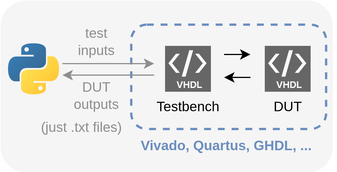
The basic principle is this: continue using VHDL testbenches, just keep the inputs given to the device under test (DUT) and the outputs collected from it in an intermediate format. This way, we can control the input-output with any language that can write-read the intermediate format, and establish a scalable simulation-based verification environment.

This article shows and exemplifies one of the simplest and most understandable ways to do this:

Write the input vector from Python to inputs.txt file,
Read it with the VHDL testbench and feed it to the DUT, write the output vector to outputs.txt file,
Read outputs.txt in Python and analyze it.

Method

When testing a module developed in VHDL, we develop testbenches in a language according to the chosen verification method, and then we create verification vectors (input + expected output) for various scenarios and feed them to the DUT through those testbenches.

It is also possible to define these input-output vectors in a language like VHDL, just like the DUT itself, but writing a module that generates realistic data in a hardware design language like VHDL would, of course, be a project in itself. We mostly do this work through ready-made libraries and simulators in environments like C++, Python, MATLAB.

Let's evaluate this over a simple DUT example: a single-channel, fixed-point, FIR low-pass filter that accepts 16-bit input-output. The details of the filter are not very important for this article, but you can find the source codes of both it and all parts related to this example in the sobulabs/vhdl-basic-sil-fir repository. We can assume that such a filter has an entity definition like this:

entity fir is
    Generic (FILTER_TAPS  : integer := 19;
             INPUT_WIDTH  : integer := 16; 
             COEFF_WIDTH  : integer := 16;
             OUTPUT_WIDTH : integer := 16 );
    Port (clk    : in STD_LOGIC;
          data_i : in STD_LOGIC_VECTOR (INPUT_WIDTH-1 downto 0);
          data_o : out STD_LOGIC_VECTOR (OUTPUT_WIDTH-1 downto 0) );
end fir;

Let's assume our VHDL testbench that will communicate with .txt files via Python is connected to this entity as data_i <= data_in and data_o <= data_out. Under the constant sampling frequency assumption, let's assume that the inputs needed to test this filter will be generated on the Python side as a 1D vector and written to a text file. For example, it could simply be a chirp generation like the following:

import numpy as np
from scipy.signal import chirp

# File paths
input_file  = "./Filter_input.txt"
output_file = "./Filter_output.txt"
tcl_script  = "./run_tb.tcl"
vivado_path = "/home/buraksoner/Tools/Xilinx/Vivado/2023.2/bin/vivado"  # Replace with your Vivado installation path

def generate_q_chirp(startfreq_hz, stopfreq_hz, clockfreq_hz, t_stop_ns, bitwidth, method="linear"):
    num_pts     = int(t_stop_ns/(1e9/clockfreq_hz));
    t = np.linspace(0, t_stop_ns/1e9, num_pts) # 0=t_start. Every tick in t corresponds to one clock cycle in the testbench
    x = chirp(t, f0=startfreq_hz, f1=stopfreq_hz, t1=t_stop_ns/1e9, method=method);
    x_int = np.floor(2**(bitwidth-1)*x) 
    return x_int

def write_to_input_file(signal, file_path):
    with open(file_path, "w") as file:
        for value in signal:
            file.write(f"{str(value.astype(np.int16))}\n")

def read_from_output_file(file_path):
    with open(file_path, "r") as file:
        data = file.readlines()
    return [int(line.strip()) for line in data]

# Generate
clk_freq    = 120e6;
t_stop_ns   = 0.5e6;
chirp_start_freq_hz = 0.5e6; # our LPF has a cutoff at 3 MHz, we're sweeping from 1 to 5 to see the drop in power
chirp_stop_freq_hz  = 5.5e6;
bitwidth = 16;
chirpsignal = generate_q_chirp(chirp_start_freq_hz, chirp_stop_freq_hz, clk_freq, t_stop_ns, bitwidth, method="linear")

write_to_input_file(chirpsignal, input_file)

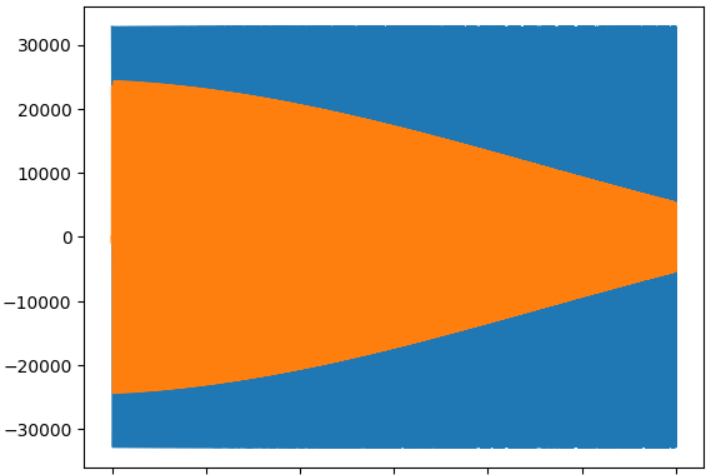
We know what should happen when this chirp is fed to our FIR filter: we expect to see high amplitude output at low frequencies (at the beginning of the simulation), and lower amplitude output as the frequency increases over time.

Now let's look at the part on the VHDL testbench side that will read Filter_input.txt and generate Filter_output.txt based on the input passed through the DUT (to keep it short, let's skip other details of the testbench, you can check them in the repo, this is only the part that reads the text file, feeds it to the DUT, and writes what comes from the DUT back to the text file):

...
    process(clk)       
        file     input_file  : text is in INPUT_FILE_NAME;
        variable input_line  : line; 
        file     output_file : text is out OUTPUT_FILE_NAME;         
        variable output_line : line;    
        variable int_input_v : integer := 0;       
        variable good_v      : boolean;                
    begin        
        if rising_edge(clk) then
            if (not endfile(input_file)) then
                write(output_line, to_integer(signed(data_out)), left, 10);
                writeline(output_file, output_line);        
                readline(input_file, input_line);
                read(input_line, int_input_v, good_v);
                int_input_s <= int_input_v;
            else
                assert (false) report "Reading operation completed!" severity failure;
            end if;
            data_in <= shift_right(to_signed(int_input_s, data_in'length), 0);
        end if;
    end process;
...

With the Filter_input.txt file generated by Python and this testbench, the DUT is now ready for simulation with the input vector. You can run this simulation through your preferred tool (Vivado, Quartus, GHDL, ...) and obtain the Filter_output.txt file. In this example, I used Vivado in "batch" mode, i.e., from the terminal via a TCL file, so I was able to start Vivado's simulator via the subprocess library on the Python side and have it generate Filter_output.txt.

We can also read the output as follows:

output_signal = read_from_output_file(output_file)
plt.plot(chirpsignal)
plt.plot(output_signal)

and we can observe the expected result as below:

FIR Low-pass Filter Chirp Test Result

Discussion / Conclusion

The development-test method introduced in this article is definitely not the most advanced method in this industry, nor is it suitable for most large-scale projects, and we have no intention of opposing methodologies like OSVVM / UVM / UVVM. However, considering all the "entry barriers" that someone starting to work with FPGAs from scratch, students, etc. will encounter, it is obvious that such a simple method will be useful and "debuggable" (in the worst case, we can open the .txt file and check if the samples are correct!). The benefit of simplified "quick trial" methods is actually obvious for experienced developers as well. When we want to quickly prototype an idea, understand how much quantization/compression losses will be when transitioning to VHDL/fixed point, etc., this is quite a quick testing ground.

Hope it's useful.

^† In the reports regularly published by Siemens and the Wilson Research Group measuring industry trends in the functional verification field, it is clear that verification efforts cover more than half of projects in terms of workforce and time. There has been an increasing trend since 2012.

Bu yazı, VHDL tabanlı algoritma geliştirmesi yapanlar için çok basit, erişilebilir ve anlaşılabilir bir Python-tabanlı "yazılım döngüde" (SiL) doğrulama metodunu anlatıyor. Öğrenciler, alana yeni girenler, gömülü sistemlerden FPGA'e geçiş yapma hazırlığındaki girişimler gibi gruplar için, OSVVM, UVM, cocotb benzeri profesyonel doğrulama araçlarının detaylarında kaybolmadan elinizi kirletmenin bir yolu da denebilir.

Motivasyon

FPGA-ASIC tabanlı geliştirme projelerinde doğrulama eforları tasarım eforlarından daha fazla zaman ve kaynak alıyor^†. OSVVM, UVM, cocotb gibi farklı dilleri hedefleyen profesyonel doğrulama araçları da buna orantılı olarak giderek gelişiyorlar. Fakat bu profesyonel araçları kullanmak, öğrenciler, alana yeni girenler, gömülü sistemlerden FPGA'lere geçiş yapma hazırlığındaki girişimler gibi gruplar için iyi bir seçenek değil.

Bu profesyonel araçların hepsinde aşağıdaki "bariyerlerden" en az bir tanesi mevcut:

Uyumluluk sıkıntısı: kullanılan EDA programlarıyla uyumlulukları kısıtlı,
Ölçeklenebilirlik sıkıntısı: artık çoğu yüksek başarımlı simülatör Python / MATLAB gibi ortamlarda, ve bu araçlar genelde diller arası geçiş sağlamıyorlar,
Öğrenim zorluğu: aracın kendisini öğrenmek başlı başına VHDL'de algoritma geliştirmekten ayrı bir iş (şirketlerin ayrı UVM takımları bile oluyor),
Fiyat sıkıntısı: kısaltmaların sonundaki M harfi, yani metodoloji ücretsiz tabii ki, fakat onların kullandığı araçlar genel olarak çoğu grup için erişilemez durumda.

Büyük / oturmuş ekipler için bu araçları kullanmanın vazgeçilemez artıları tabii ki var, ama küçük / yeni ekiplerin işini görebilecek, ve doğrulama metodolojisini öğrenmeye yardımcı olacak çok daha basit bir opsiyon da mevcut.

Temel prensip şu: VHDL testbench'lerini kullanmaya devam et, sadece test edilen cihaza (DUT) verilen girdileri ve ondan geri toplanan çıktıları bir ara formatta tutalım. Bu şekilde ara formatı yazıp-okuyabilen herhangi bir dil ile girdi-çıktı kontrolünü sağlayalım, ve ölçeklenebilir bir simülasyon-tabanlı doğrulama ortamı kuralım.

Bu yazı bunu yapmanın en basit ve anlaşılabilir yollarından birini gösteriyor ve örnekliyor:

Python'dan inputs.txt dosyasına girdi vektörünü yaz,
VHDL testbench'iyle oku ve DUT'a besle, çıktı vektörünü outputs.txt dosyasına yaz,
Python'da outputs.txt'i oku ve analiz et.

Metod

VHDL'de geliştirilen bir modülü test ederken seçilen doğrulama metoduna göre bir dilde testbench'ler geliştiriyoruz, sonra da türlü senaryolar için doğrulama vektörlerini (girdi + beklenen çıktı) oluşturup, o testbench'ler vasıtasıyla DUT'a besliyoruz.

Bu girdi-çıktı vektörlerini de aynı DUT'un kendisi gibi VHDL gibi bir dilde tanımlamak da mümkün, ama realistik veriyi yaratan bir modülü VHDL gibi bir donanım tasarım dilinde yazmak tabii ki başlı başına bir proje olur. Çoğunlukla bu işi C++, Python, MATLAB gibi ortamlardaki hazır kütüphaneler ve simülatörler vasıtasıyla yapıyoruz.

Basit bir DUT örneği üstünden bunu değerlendirelim: tek kanallı, fixed-point çalışan, 16-bit girdi-çıktı kabul eden bir FIR alçak geçirgen filtre. Filtrenin detaylarının bu yazı için çok önemi yok, ama hem onun hem de bu örnekle ilgili tüm parçaların kaynak kodlarını sobulabs/vhdl-basic-sil-fir repo'sunda bulabilirsiniz. Böyle bir filtrenin şöyle bir entity tanımı olduğunu kabul edebiliriz:

entity fir is
    Generic (FILTER_TAPS  : integer := 19;
             INPUT_WIDTH  : integer := 16; 
             COEFF_WIDTH  : integer := 16;
             OUTPUT_WIDTH : integer := 16 );
    Port (clk    : in STD_LOGIC;
          data_i : in STD_LOGIC_VECTOR (INPUT_WIDTH-1 downto 0);
          data_o : out STD_LOGIC_VECTOR (OUTPUT_WIDTH-1 downto 0) );
end fir;

Python'la .txt dosyaları üstünden iletişecek olan VHDL testbench'imiz bu entity'ye data_i <= data_in ve data_o <= data_out şeklinde bağlanıyor olsun. Sabit örnekleme frekansı varsayımı altında bu filtreyi test etmek için gerekli girdilerin bir 1D vektör olarak Python tarafında üretilip, bir text dosyasına yazılacağını varsayalım. Mesela aşağıdaki gibi basitçe bir chirp üretimi olabilir:

import numpy as np
from scipy.signal import chirp

# File paths
input_file  = "./Filter_input.txt"
output_file = "./Filter_output.txt"
tcl_script  = "./run_tb.tcl"
vivado_path = "/home/buraksoner/Tools/Xilinx/Vivado/2023.2/bin/vivado"  # Replace with your Vivado installation path

def generate_q_chirp(startfreq_hz, stopfreq_hz, clockfreq_hz, t_stop_ns, bitwidth, method="linear"):
    num_pts     = int(t_stop_ns/(1e9/clockfreq_hz));
    t = np.linspace(0, t_stop_ns/1e9, num_pts) # 0=t_start. Every tick in t corresponds to one clock cycle in the testbench
    x = chirp(t, f0=startfreq_hz, f1=stopfreq_hz, t1=t_stop_ns/1e9, method=method);
    x_int = np.floor(2**(bitwidth-1)*x) 
    return x_int

def write_to_input_file(signal, file_path):
    with open(file_path, "w") as file:
        for value in signal:
            file.write(f"{str(value.astype(np.int16))}\n")

def read_from_output_file(file_path):
    with open(file_path, "r") as file:
        data = file.readlines()
    return [int(line.strip()) for line in data]

# Generate
clk_freq    = 120e6;
t_stop_ns   = 0.5e6;
chirp_start_freq_hz = 0.5e6; # our LPF has a cutoff at 3 MHz, we're sweeping from 1 to 5 to see the drop in power
chirp_stop_freq_hz  = 5.5e6;
bitwidth = 16;
chirpsignal = generate_q_chirp(chirp_start_freq_hz, chirp_stop_freq_hz, clk_freq, t_stop_ns, bitwidth, method="linear")

write_to_input_file(chirpsignal, input_file)

Bu chirp'ün FIR filtremize verildiğinde olması gerekeni biliyoruz: düşük frekanslarda (simülasyonun başlarında) yüksek genlikte, ilerleyen zamanlarda ise frekans yükseldikçe daha düşük genlikte bir çıktı görmeyi bekliyoruz.

Şimdi de VHDL testbench tarafında Filter_input.txt i okuyup Filter_output.txt i DUT'tan geçen girdiye göre üretecek olan parçaya bakalım (kısa tutmak adına testbench'in diğer detaylarını es geçelim, onlara repo'dan bakabilirsiniz, bu yalnızca text dosyasını okuyup, DUT'a besleyen, ve DUT'tan geleni de geri text dosyasına yazan kısım):

...
    process(clk)       
        file     input_file  : text is in INPUT_FILE_NAME;
        variable input_line  : line; 
        file     output_file : text is out OUTPUT_FILE_NAME;         
        variable output_line : line;    
        variable int_input_v : integer := 0;       
        variable good_v      : boolean;                
    begin        
        if rising_edge(clk) then
            if (not endfile(input_file)) then
                write(output_line, to_integer(signed(data_out)), left, 10);
                writeline(output_file, output_line);        
                readline(input_file, input_line);
                read(input_line, int_input_v, good_v);
                int_input_s <= int_input_v;
            else
                assert (false) report "Reading operation completed!" severity failure;
            end if;
            data_in <= shift_right(to_signed(int_input_s, data_in'length), 0);
        end if;
    end process;
...

Python tarafından üretilen Filter_input.txt dosyası ve bu testbench ile DUT artık girdi vektörüyle simülasyona hazır. Tercih ettiğiniz araç üstünden bu simülasyonu koşturup Filter_output.txt dosyasını elde edebilirsiniz (Vivado, Quartus, GHDL, ...). Bu örnekte ben Vivado'yu "batch" modunda, yani terminalden bir TCL dosyası vasıtasıyla kullandım, o yüzden Python tarafında subprocess kütüphanesi vasıtasıyla Vivado'nun simülatörünü ayağa kaldırıp, Filter_output.txt i oluşturtabildim.

Çıktıyı da aşağıdaki gibi okuyabiliyoruz:

output_signal = read_from_output_file(output_file)
plt.plot(chirpsignal)
plt.plot(output_signal)

ve aşağıdaki gibi beklediğimiz sonucu gözlemleyebiliyoruz:

FIR Low-pass Filter Chirp Test Result

Tartışma / Sonuç

Bu yazıda tanıtılan geliştirme - test metodu bu sektördeki en gelişmiş metod kesinlikle değil, çoğu büyük çaplı proje için de uygun değil, OSVVM / UVM / UVVM gibi metodolojilerin karşısına çıkma gibi bir amacımız yok. Fakat FPGA'lerle çalışmaya sıfırdan başlayacak birinin, öğrencilerin vs. karşılaşacağı tüm "giriş bariyerleri" göz önünde bulundurulduğu zaman bu kadar basit bir metodun faydalı ve "debuggable" olacağı aşikar (en kötü ihtimalle açıp .txt dosyasındaki örnekler doğru mu diye bakabiliyoruz!). Basitleştirilmiş "hızlı deneme" metodlarının faydası tecrübeli geliştiriciler için de aslında aşikar. Hızlıca bir fikri prototiplemek, VHDL / fixed point'e geçince quantization / sıkıştırma kayıplarının ne kadar olacağını anlamak vs. istediğimizde de bu oldukça hızlı bir deneme tahtası.

Faydalı olması ümidiyle.

^† Siemens ve Wilson Research Group'un düzenli olarak yayınladığı fonksiyonel doğrulama (Functional Verification) alanında sektör trendlerini ölçümleyen raporlarda, doğrulama eforlarının projelerin iş gücü ve zaman olarak yarısından fazlasını kapladığı açık. 2012'den beri de giderek artan bir trend sözkonusu.

View on GitHub

arrow_back Back to Blog